Jonathan’s Discovery
Jonathan Kirk is a young man who has been using Zometool and vZome since he was nine or ten years old. He has a lot of experience with building real and virtual models of 4D polytope projections. Last year, he put that experience to work in vZome to construct a previously unknown CRF polytope, as a 3D projection, just using his considerable intuition and exceptional visualization skills. Let that sink in: he used a 2D view of a 3D projection to intuit the configuration of a 4D polytope.
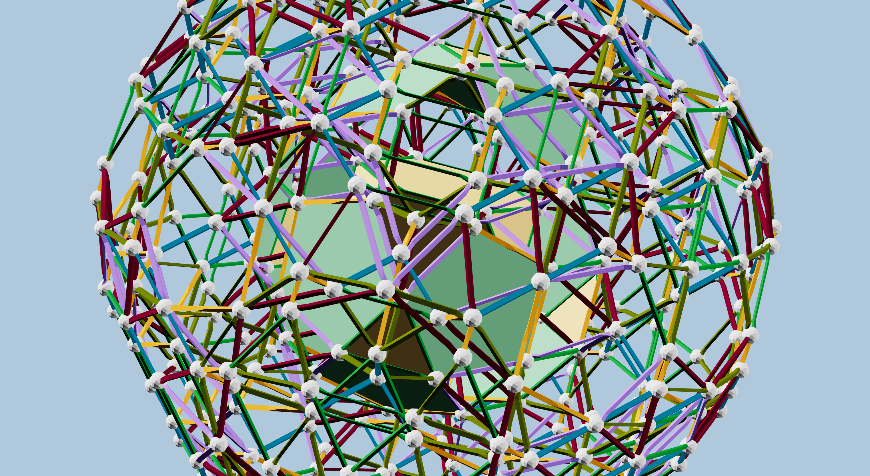
In Figure 1, have added panels to Jonathan’s design, to highlight the truncated tetrahedron seed he started with, and the four J92 Johnson solids surrounding it. This was his initial inspiration, based on the hexagonal faces of those two kinds of polyhedra. Then he continued to find reasonable ways to fill in gaps, while always respecting the tetrahedral overall symmetry of the projection, and the foreshortening always found in these orthogonal projections of 4D polytopes.
This is a remarkable achievement, made even more so because he did not use regular Zome struts! He wanted to build something with tetrahedral symmetry, so he knew he needed to work in this octahedral system, familiar to him from looking at projections of other 4D polytopes. Not only does this system use a subset of the possible green strut directions, it also uses subsets of the maroon, lavender, and olive strut directions.
The polytope has several types of cells:
- J92s
- J91s
- J63s
- icosidodecahedra
- truncated tetrahedra
- tetrahedra
- octahedra
- triangular prisms
These all satisfy the requirements for being convex and having regular faces, and constitute a mix of Platonic, Archimedean, and Johnson polyhedra.
Verification
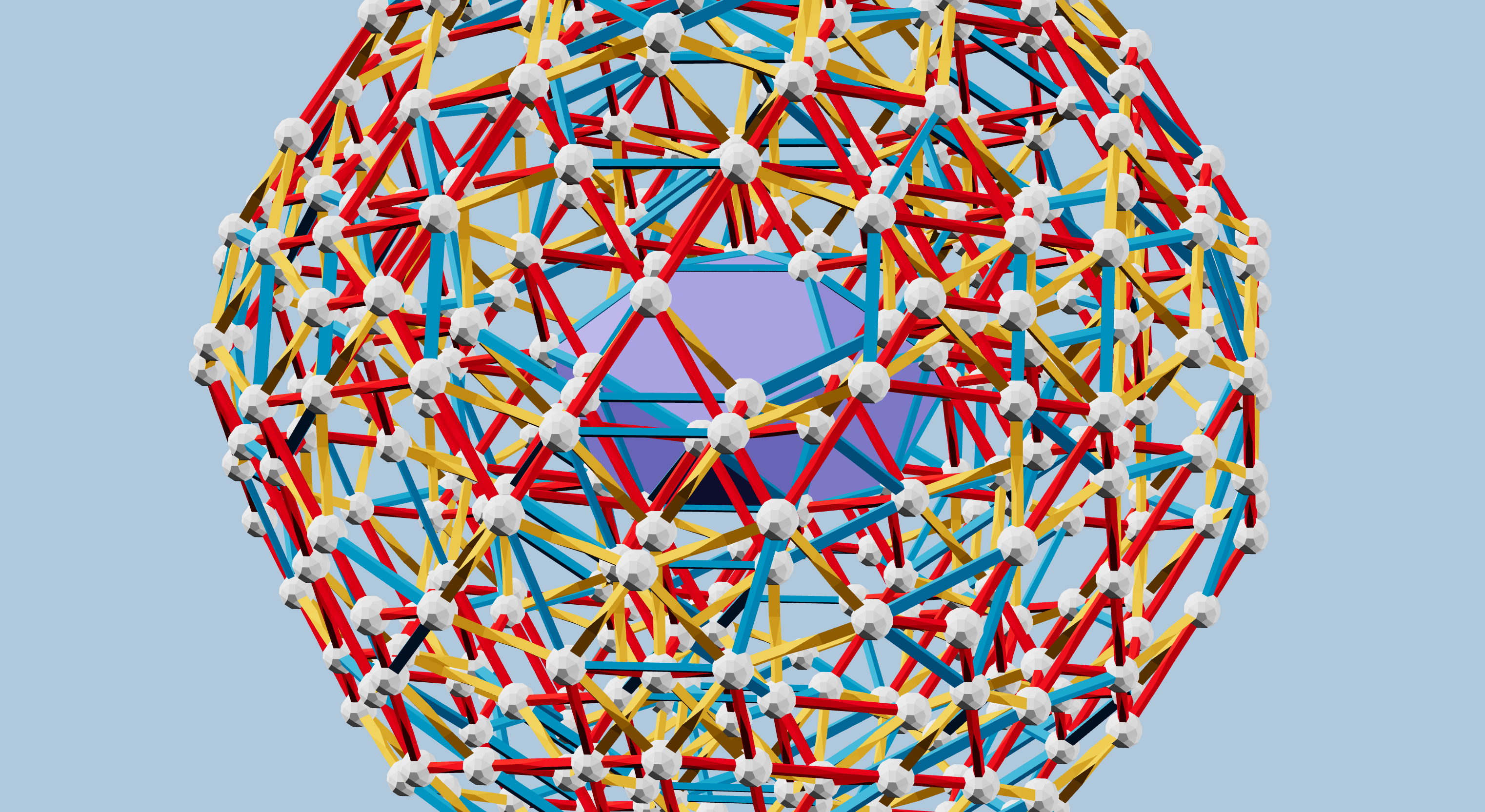
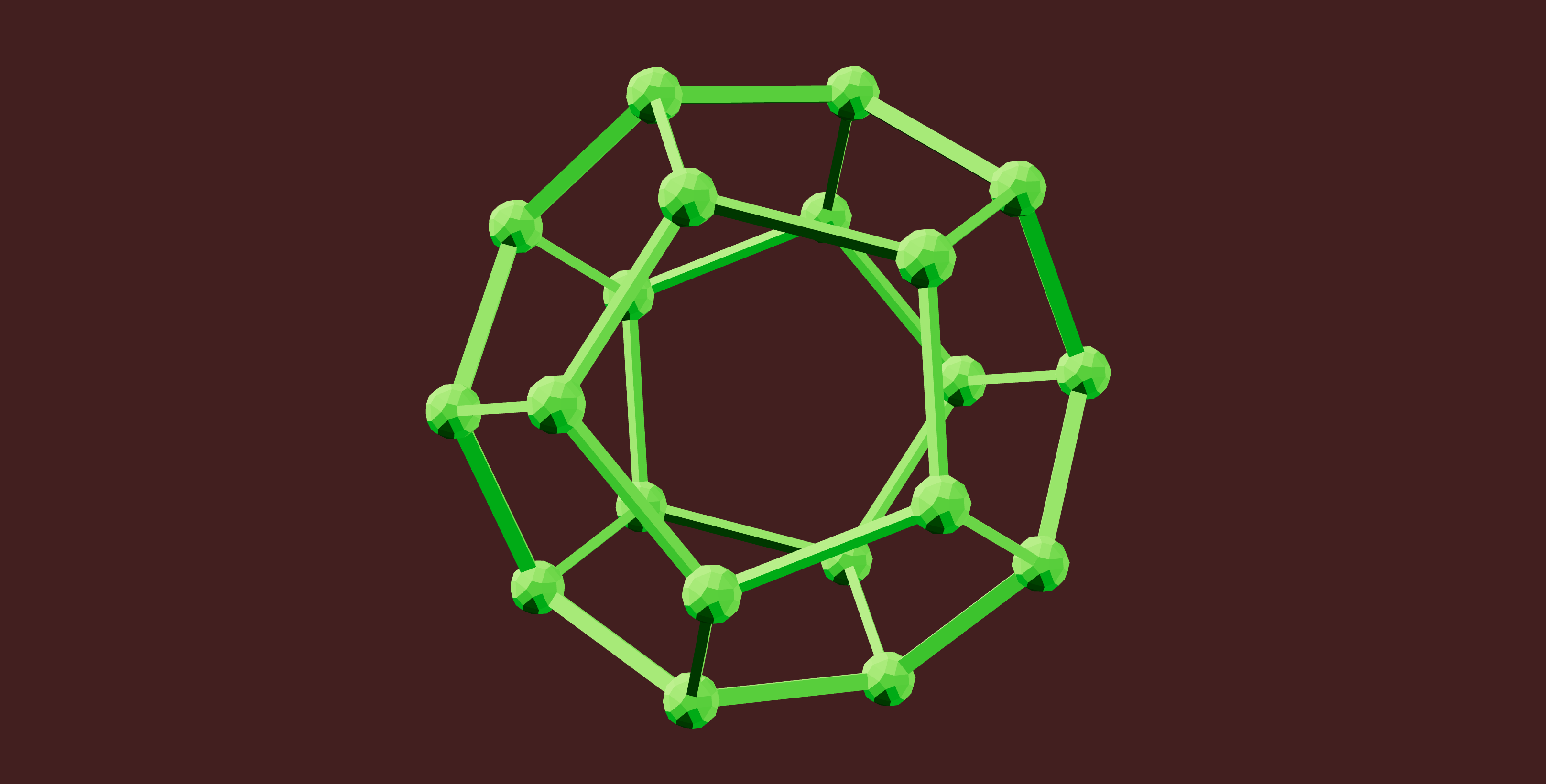
Now, just because he was able to create this 3D design, which follows all the usual patterns for a 4D polytope projected to 3D, there is no guarantee that the 4D polytope actually works. His first idea for verifying the polytope was to find another projection to 3D. Between us, we were able to reproduce the adjacency defined in his projection, but in the standard Zometool red-yellow-blue struts, in three different projections, each with a different cell at the center, though I only really completed one of them, seen here in Figure 2.
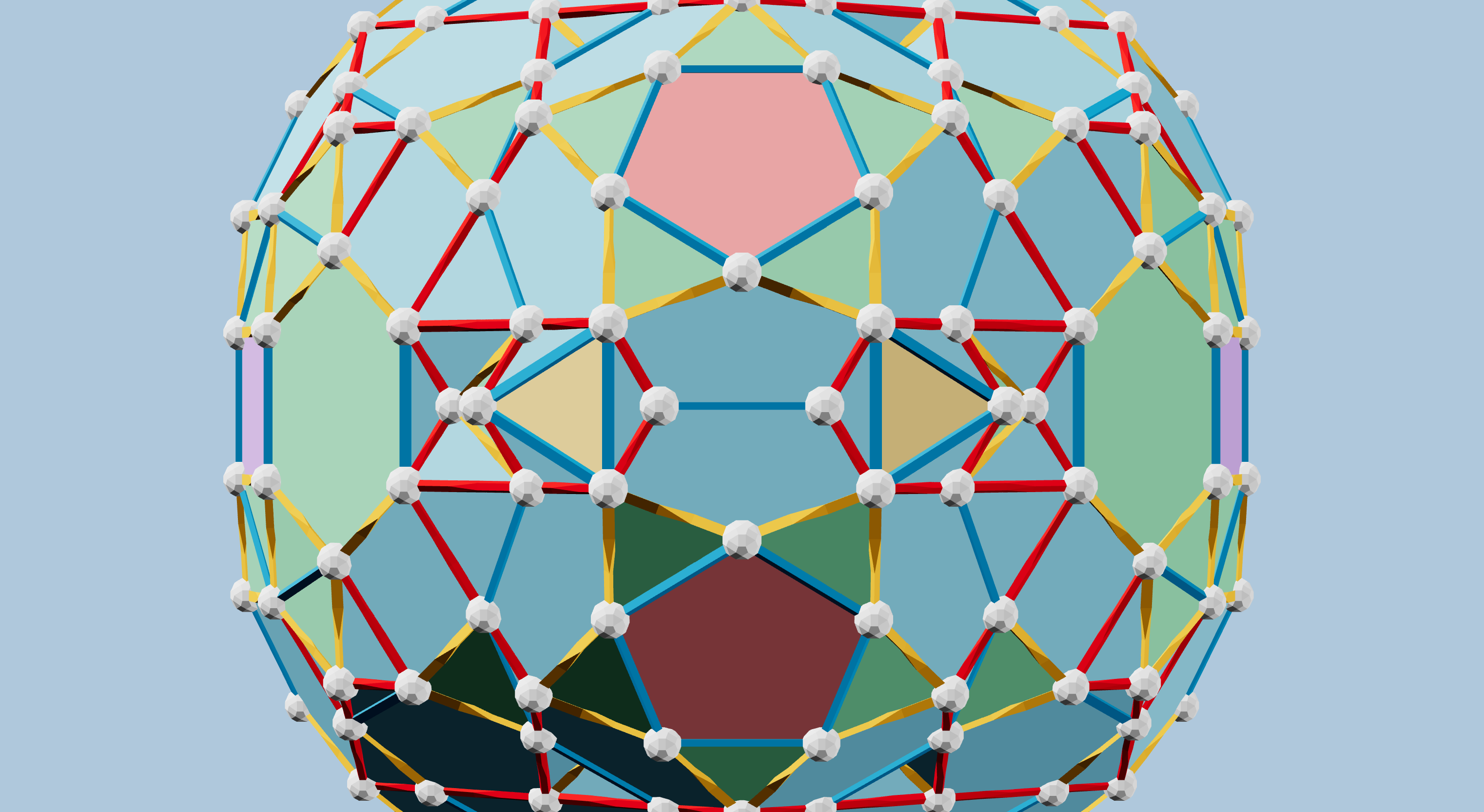
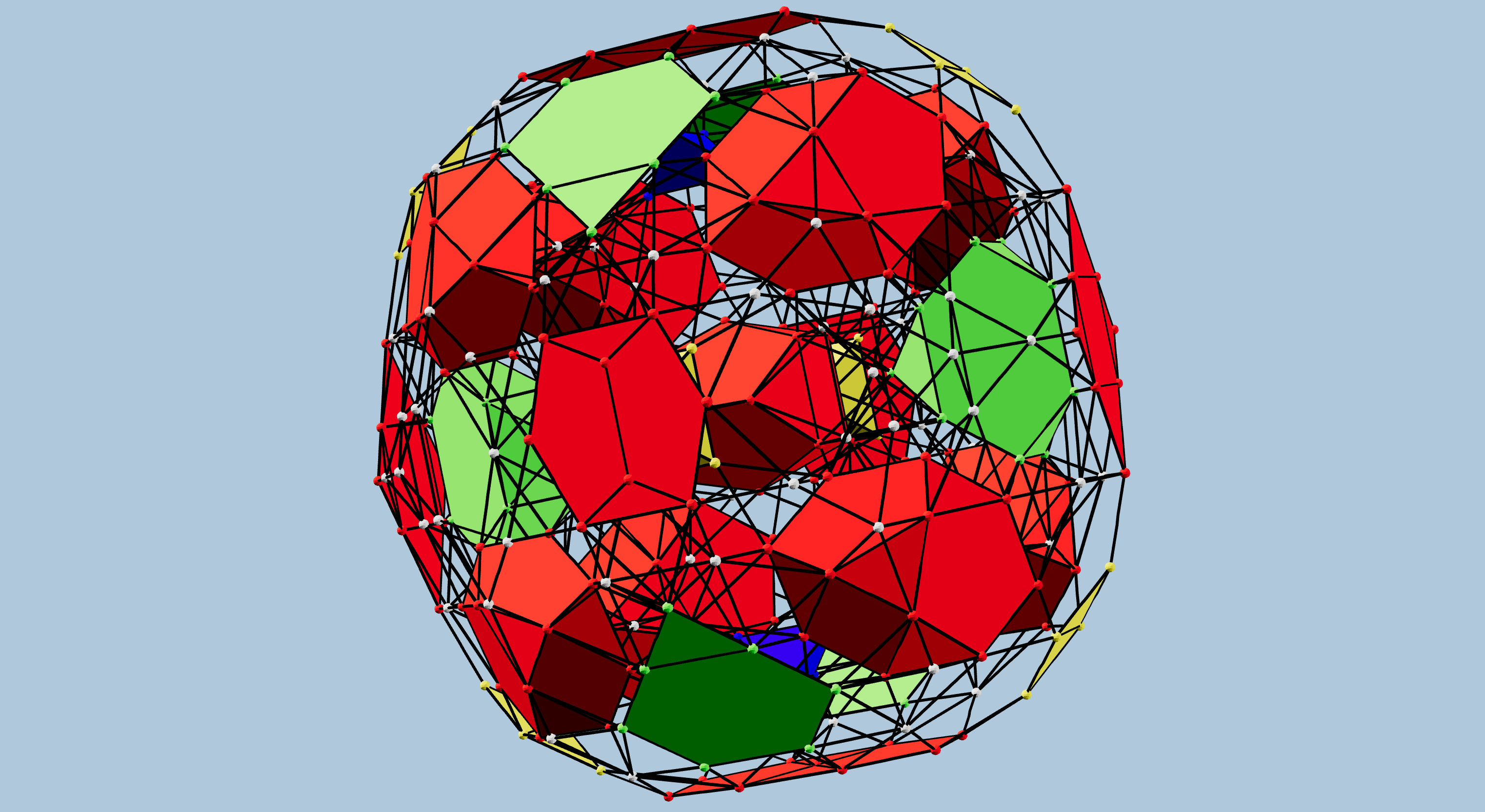
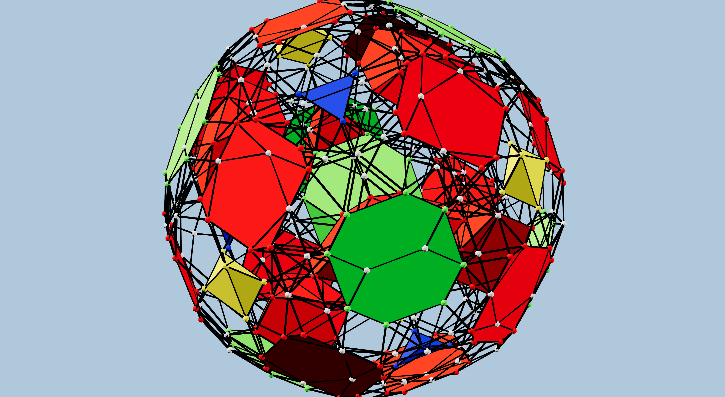
Figures 3 and 4 show two more hand-built partial projections, illustrating some additional centers of tetrahedral projection. These use the same strut colors as Jonathan’s original, necessarily.
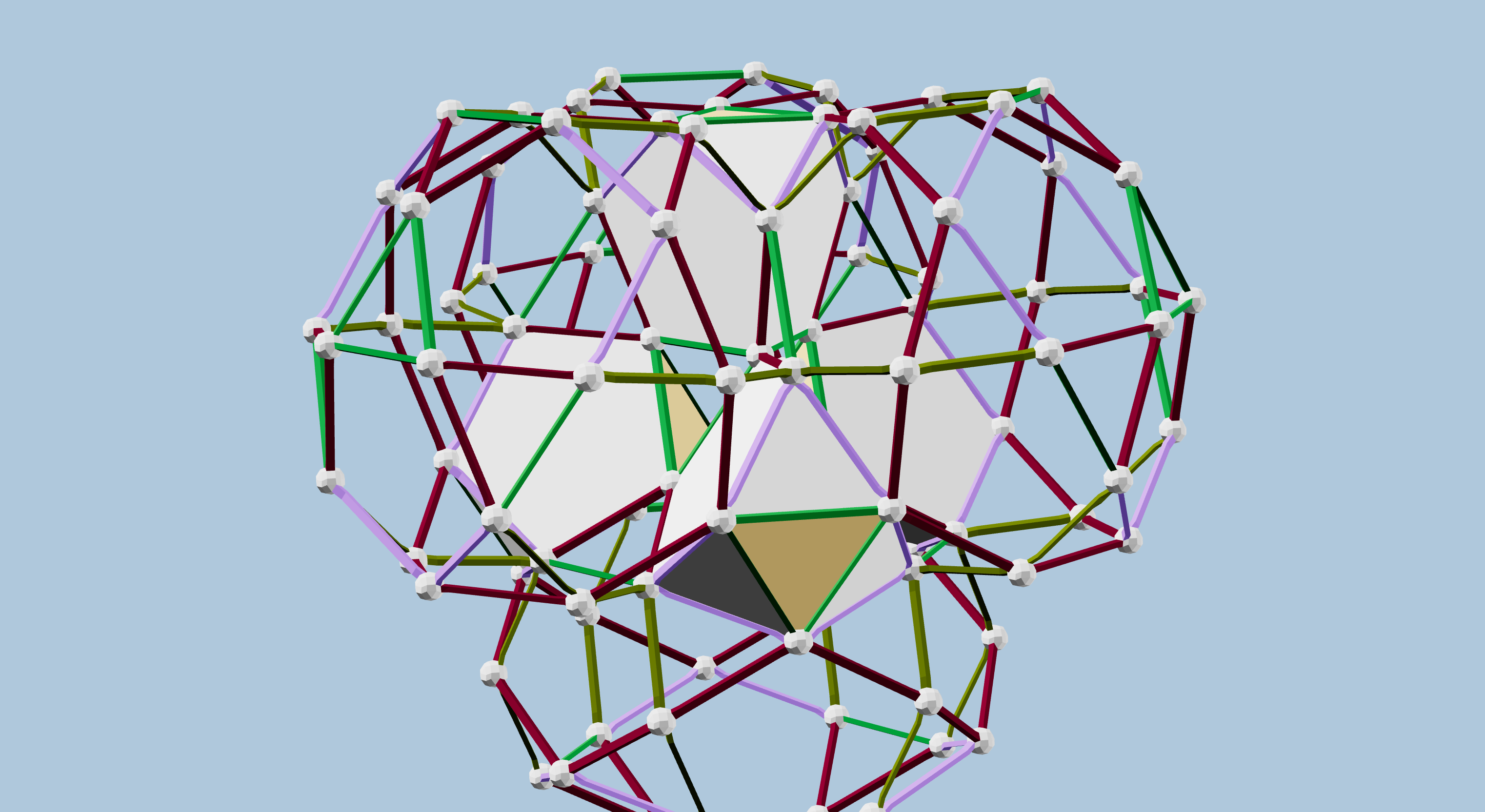
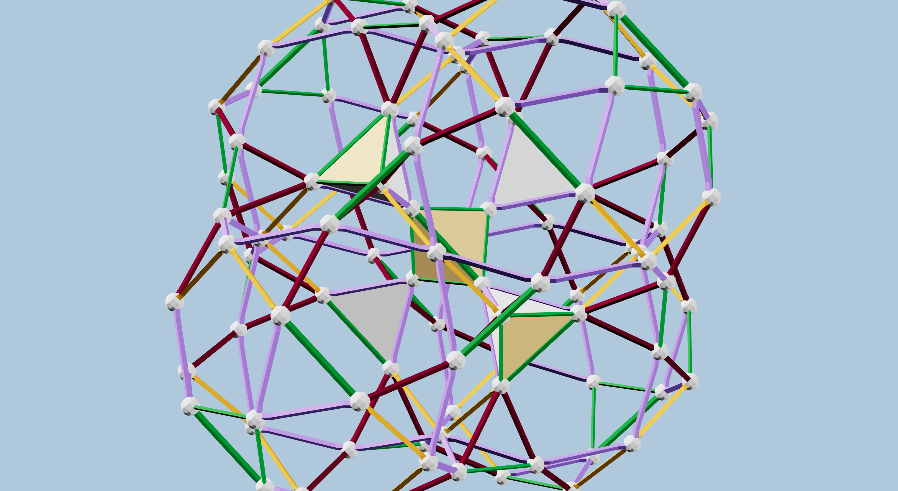
Our ability to create several partial projections, using strut color combinations familiar from projecting other 4D polytopes like the 120-cell and 600-cell, served as very compelling, yet still circumstantial, evidence that the projections represented a legitimate CRF polytope.
Nonetheless, I promised Jonathan that I would try to reconstruct the full 4-dimensional vertex dataset. In the general case, reconstructing a 4D object from a 3D projection is impossible, since information is lost. However, this kind of polytope lets us make several assumptions that I believed would allow it. The convexity of the polytope and its 3D cells and 2D faces is one such attribute. Another is the planarity of faces, and finally, the uniformity of edge lengths is central.
I have succeeded in this effort, recreating 4D coordinates for all of the vertices. I started from my most complete and most symmetric red-yellow-blue projection, with a J91 (bilunabirotunda) at the center. (See Figure 6 below.)
The algorithm is fairly simple, but hard to visualize, so I’ve illustrated it in Figure 5 using a 2D projection of a 3D polyhedron. The principles are all the same. The algorithm starts by identifying some parts of the projection that are already in the Z=0 plane. Adjacent to those, we can use the Pythagorean theorem to derive the Z coordinate for the next few vertices. We do have to make a choice, here, for which Z value to use, positive or negative, so we choose positive values consistently.
Finally, we enter the main iteration of the algorithm. In this phase, we schedule faces for which we already have two edges resolved to 3D. For each such face, we find three vectors to vertices in the projection, and three more to the corresponding 3D vertices. These six linearly independent vectors uniquely define a linear mapping that “unprojects” the face to 3D, simply by mapping one 2D plane to another. Note that this mapping is only valid for that particular face; for each face we must fine the specific mapping, and recover the Z values for all the vertices of the face.
There is one trick here that I learned from David Richter: assign the projection a Z value of one, or really any non-zero number, to be certain that our three vectors will not be coplanar.
The algorithm recovers the higher-dimensional data for just one half of the entire polytope, since we used only positive Z values. The final steps require a reflection in the Z=0 plane, then computing the convex hull from the full set of vertices.
The algorithm for 3D to 4D is essentially identical. I was able to reflect the half-polytope data
in the projection hyperplane, topology and all, to nearly complete the 4D polytope.
From that data, I generated this 4D OFF file file, and shared it on the Polytope Discord server.
One user ran it through Stella4D, and produced a table of cell neighborhood types, and confirmation that
the polytope is convex.
I then ran the vertex data through the free qhull command-line tool;
that tool has various output formats that let me regenerate the full topology of edges, faces, and cells,
now including all of the cells that had been flattened in the original projection, and thus missing from my initial topology.
Another user on the same Discord server started from Jonathan’s original projection 3D data, and performed some computation analogous to mine. They generated a second 4D data set, though starting from a different set of 4D basis vectors.
More Visualizations
With the 4D data in hand, we can create a variety of projections.
I am trying to produce some better views of Jonathan’s polytope, including the ability to dynamically change the projection and to “explode” the projected cells to make the structure easier to see. I have some initial results in an Observable notebook that I will continue to improve. For now, you can play with the exploding cells, though the interface is a bit clunky.
I am also working on another Observable notebook derived from this one. It will use a stereographic projection and the color coding seen in figures 7 and 8, and allow arbitrary 4D rotations to explore the polytope. Again, stay tuned.
If you know how to import vZome’s Simple Mesh JSON format, you can try your hand at different projections in vZome. You can download the JSON file here.